Let me tell you a story about adulthood. It all started when I decided to understand how loans actually work instead of just signing up for one and hoping the bank was feeling generous. Spoiler alert: they weren’t.
So I did what any spreadsheet-loving, financially-curious human would do: I opened Excel and made an amortization table. And as it turns out? It was kind of empowering, and way more satisfying than just watching my monthly payments vanish into the void.
If you’re wondering how to build one too, grab your loan details and an energy drink. This is about to get responsibly nerdy.
What Is an Amortization Table, Anyway?
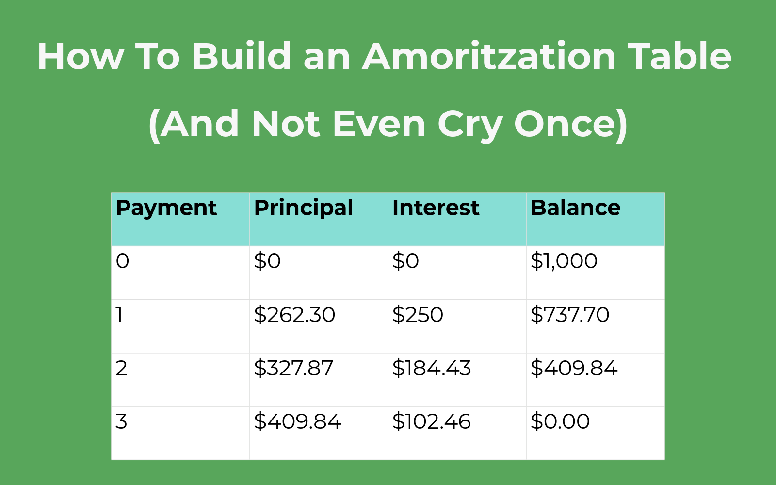
Think of an amortization table as a very detailed receipt for your loan. It breaks down every single payment over time, showing you how much goes toward interest, how much pays down your principal, and what’s left after each payment.
It’s like watching your debt shrink in slow motion, one row at a time.
Step 1: Gather the Basics
To get started, you’ll need:
Loan Amount (also called the principal), Annual Interest Rate Loan Term (in years), and the Payment Frequency (we’ll assume monthly here)
For this walkthrough, let’s say:
Loan Amount = $10,000, Interest Rate = 5%, and Term = 3 years Monthly payments
Open Excel and enter those values in clearly labeled cells, like: A1: Loan Amount B1: 10000 A2: Annual Interest B2: 0.05 A3: Term in Years B3: 3 A4: Payments/Year B4: 12
Step 2: Calculate Monthly Payment Using PMT
Next, use Excel’s PMT function to calculate the monthly payment: =PMT(rate, nper, pv)
In our case: =PMT(B2/B4, B3*B4, -B1)
Place that in cell B5, and label it “Monthly Payment” in A5. The negative sign is just so Excel gives us a positive number (pfft computers, am I right?).
Step 3: Set Up the Table Headers
Starting in A7, label your columns: Payment #; Payment; Interest; Principal; Balance
Now the magic begins.
Step 4: Build the First Row of the Amortization Table
Row 8 will be your starting point:
In E7, enter =B1 so the balance starts at the full loan amount.
- A8: 1 (Payment #1)
- B8: =$B$5 (Monthly payment)
- C8: =E7*$B$2/$B$4 (Interest for the month; reference E7 as the balance from the row above, set E7 to the loan amount manually)
- D8: =B8-C8 (Principal paid this month)
- E8: =E7-D8 (Remaining balance)
Step 5: Fill Down the Rows
Now drag that row down for as many periods as the loan lasts. That’s B3 * B4 or 36 rows for a 3-year loan with monthly payments.
Excel will do the math for each month: payment stays the same, interest decreases over time, and principal increases while the balance drops, row by row.
When the final balance hits zero (or close to it, rounding can make it slightly off), your table is complete!
Bonus Features for Spreadsheet Overachievers
Want to spice things up? Try adding:
Conditional formatting to highlight the final payment A line chart to visualize principal vs. interest over time A separate input box for extra payments if you want to simulate paying off your loan faster (and feel superior)
Why This Is Worth Doing
Besides giving you warm, budget-conscious feelings, building an amortization table in Excel helps you:
Understand how interest eats into your early payments See how much total interest you’re paying (ouch) Plan for future payments or early payoffs
It’s also a great excuse to tell people you “ran a financial model” over the weekend. Impressively nerdy.
Final Thoughts: You + Excel = Loan Payoff Power Couple
Creating an amortization table in Excel might seem intimidating, but it’s actually a brilliant way to take control of your financial life. Once you build one from scratch, you’ll never look at loan documents the same way again. You’ll know where your money’s going, and that’s half the battle.
So go ahead. Fire up Excel, crunch those numbers, and enjoy watching your loan balance go down. One glorious, calculated row at a time.